Abstract
Exoplanets are of great interest due to the prospects of them harboring life. As radio telescopes become more sensitive, there have been efforts to detect exoplanets via electron-cyclotron maser instability (ECMI), providing a new way to detect exoplanets. This reveals information about their magnetic fields and stellar flux previously unobtainable from other exoplanet detection methods, hinting at the habitability of these exoplanets. We outline the search process and results for a crossmatch between Hot Jupiters in the NASA Exoplanet Archive and ASKAP survey data for the southern sky, searching for candidate systems with radio-emitting exoplanets. The crossmatching resulted in two matches between radio sources and exoplanets in candidate systems Proxima Centauri and Au Microscopii, giving readings within the theoretical range of radio flux produced by exoplanet ECMI. More observations on these candidate systems are needed to determine whether these radio flux readings are caused by ECMI or other factors.
1. Introduction
1.1 Exoplanets
Exoplanets are planets that exist outside our solar system, either orbiting other stars or as rogue planets untethered to any star. In particular, exoplanets orbiting stars are of great interest due to the possibility of them being habitable for life. As of 26 May 2024, there were 5,632 known confirmed exoplanets listed in NASA’s Exoplanet Archive, detected using various methods, each revealing information regarding the exoplanet’s parameters.
1.1.1 Exoplanet detection methods
An overview of these exoplanet detection methods is given below [8]:
- Radial velocity measurements. The gravitational pull from an exoplanet orbiting a star causes the star to orbit the center of mass of itself and its exoplanet. This displacement is measured via Doppler measurements of the star’s light. This reveals information about the exoplanet’s mass and its period, distance, and shape of its orbit around the star.
- Astrometry. This involves precise measurements of a star’s position around an exoplanet compared to the positions of other stars in the background. This reveals the same information as radial velocities, while also giving the true orientation and inclination of the exoplanet’s orbit.
- Direct imaging. This detects photons from the system, attempting to disentangle photons belonging to the exoplanet from photons belonging to the host star. It reveals the exoplanet’s spectra, allowing characterization of its atmosphere.
- Transit light curves. This measures variations in the flux of a system, indicating the presence of an exoplanet passing in front of its star from the observer’s line of sight. Combined with radial velocity data, this reveals the exoplanet’s and star’s masses and radii with a one-parameter degeneracy.
- Gravitational microlensing. This involves observing the gravitational lensing effect of a background light source caused by an exoplanet. Generally, if a planet acts as the lens, it reveals information about the ratio between the masses of the planet and star.
- Timing. Any star with observable periodic behavior can show evidence of exoplanet companions through variations in those behaviors, similar to the radial velocity, Doppler shift, and exoplanet transit methods.
1.1.2 NASA Exoplanet Archive
The NASA Exoplanet Archive is an exoplanet and stellar catalog maintained by the NASA Exoplanet Science Institute (NExScI) at Caltech. This database contains confirmed exoplanet parameters such as right ascension (RA), declination (DEC), yearly proper motion with uncertainties, and discovery characterization data such as observation epoch [1].
1.2 Detecting exoplanets via radio emission
1.2.1 Electron-cyclotron maser instability
Exoplanets with a magnetic field and a source of energetic (keV) electrons—often the solar wind from the host star—produce radio emission comparable to the host star’s radio emission, unlike optical emission. This emission occurs when energetic electrons flow along a planet’s magnetic field lines, which act as low-resistance wires. Energy in these “wires” results in visible aurora and escaping cyclotron radio emission [17]. The emission is 100% circularly polarized and theoretically should be detected at a similar level to its total-intensity emission [13].
A macroscopic empirical relationship between emitted radio power and incident solar power exists for all magnetic planets, called the radiometric Bode’s law:
Here, is the median emitted radio power, is the incident solar wind power, is the efficiency of solar-to-radio power, and is the power-law index. The relationship is used to predict the intensity of a magnetic exoplanet’s radio emission.
The maximum frequency of radio emission is proportional to the maximum planetary magnetic field strength :
Exoplanet radio emission is predicted to peak at frequencies below 10–100 MHz [17].
1.2.2 Radio emission as a detection method
As technology advances, we are becoming capable of reaching the detection threshold for exoplanet radio emission. This offers a direct detection method, unlike the indirect methods described in Section 1.1.1 [10].
Radio observations allow us to confirm whether an exoplanet has a magnetic field and constrain its strength near the surface. Circular polarization in the emission can also reveal which hemisphere is the source, alongside the plasma density in the planet’s magnetosphere [13].
Knowing exoplanet magnetic field properties helps us infer habitability. For example, we can deduce the stellar radiative flux encountered by an exoplanet in a given region around a star and determine whether it permits liquid water, assuming a rocky planet with a basic atmosphere. Magnetic field strength also tells us whether a planet can shield itself from high-energy particles from its host star [10].
1.2.3 Hot Jupiters
For radio emission to be detectable, it must be bright enough and able to propagate from the source to an observer. A lower frequency limit for this propagation is given by the characteristic plasma frequency of a plasma with number density (in ):
Radio emission at frequencies below will be absorbed by the plasma itself. If the emission frequency is below the plasma frequency of Earth’s ionosphere (a maximum of 10 MHz), it cannot be detected by ground-based telescopes [11].
Ideal candidates are Hot Jupiters: exoplanets with masses similar to Jupiter and orbital axes below 0.1 au [14]. Their proximity to host stars increases the solar wind flux through their magnetic fields. They are also predicted to have relatively strong magnetic fields , as models predict that field strength is proportional to planet mass [6]:
Distance between source and observer is another important factor because radio flux obeys an inverse-square law [10].
1.2.4 ASKAP and CASDA
The Australian Square Kilometre Array Pathfinder (ASKAP) is a radio telescope at the Murchison Radio-astronomy Observatory in Western Australia, operating from 700–1,800 MHz. The CSIRO ASKAP Science Data Archive (CASDA) provides astronomers with an interface for querying ASKAP data products [7]. ASKAP’s northern declination limit is +40 degrees, with a 2.5-arcsecond uncertainty in image pixel data [12].
1.3 Proper motion of stars
Proper motion is the apparent motion of a star in right ascension and declination across the celestial sphere, measured from the Sun’s position in arcseconds per year [16].
To crossmatch sources from different observations, their coordinates must be corrected for proper motion. Given observation epochs A and B, we determine the source position at each epoch. If the epoch-A corrected source matches another survey source at epoch A, and the epoch-B corrected source matches another source at epoch B, the same source exists in both observations [5].
We use this method to crossmatch known exoplanet positions from the NASA Exoplanet Archive with radio sources from ASKAP surveys and identify candidate systems that may contain detectable radio-emitting exoplanets.
2. Methods
2.1 Sample choice
Our initial sample came from the NASA Exoplanet Archive’s confirmed planets as of 29 April 2024. We filtered it for likely radio-emitting candidates using the criteria from Section 1.2.3: distance below 25 parsecs, chosen to reach faint luminosity limits in a reasonable amount of time [3]; declination below +40 degrees, based on ASKAP’s limit; and orbital axis at or below 0.1 au, for a better chance of interaction with magnetic planets [14].
2.2 Crossmatching algorithm
2.2.1 Technologies used
The crossmatching program was written in Python 3.10 using astropy v6.0.0, scipy v1.13.0, and astroquery v0.4.7. It crossmatches ASKAP catalogue data with the filtered NASA Exoplanet Archive data described in Section 2.1, seeking exoplanet sources corresponding to ASKAP radio sources. The main algorithm is split into Main 1A, 2A, and 3A below.
2.2.2 Filtering initial NASA data
Before crossmatching, the user authenticates their CASDA OPAL account so the program can download files for Main 2A and 3A. Duplicate planet sources are removed from the NASA data (ND), retaining the most up-to-date parameters. To simplify proper-motion correction, we keep only rows with GAIA DR2 observation times, corresponding to epoch J2015.5. The program then iterates through each source in this filtered data (FND) to seek matches in ASKAP.
Require: NASA exoplanet data CSV, ND
FND ← remove duplicate planet rows from ND
FND ← select planets with a GAIA DR2 ID
casda ← log in to CASDA OPAL
save FND as Hot_Jupiters/Filtered_NASA_only_GAIA.csv
2.2.3 Proper motion correction
For every exoplanet in FND, we query CASDA for the observation catalogue whose center coordinate is closest to the exoplanet. Using that catalogue’s observation epoch, the coordinates are corrected from J2015.5 to determine where the exoplanet was at the time of the observation.
Require: Main Algorithm Part 1 execution
for CS in FND:
BCF ← Search_Closest_Catalogue(ra, dec, casda, True)
if BCF does not exist: continue
epoch ← ending observation time (t_max) of BCF
pl_dat ← (ra, dec, pmra, pmdec, distance) from CS
pl_coord ← pl_dat at observation time J2015.5
pm_coord ← apply_space_motion(pl_coord, epoch)
add corrected RA, DEC, and epoch data to CS
save FND to NASA_with_Proper_Motion
Get_Pubdat retrieves CASDA continuum component files, selecting only released data of good or uncertain quality. For performance, the data is cached unless a refresh is requested. Our results used CASDA data retrieved on 6 May 2024.
Require: refresh
if refresh is True:
res ← CASDA catalogue continuum component files
res ← GOOD or UNCERTAIN quality, released data
pubdat ← res
save pubdat to casda_cache
else:
pubdat ← read from casda_cache
return pubdat
Because CASDA provides multiple files per observation, we select only the primary-image catalogue that sums total intensity across the processed bandwidth: .cont.taylor.0.restored.conv.components.xml. This avoids redundant downloads.
Each catalogue file is queried for its center coordinates. Files within 3 degrees of the current exoplanet are added to a candidate list. Their data is downloaded and concatenated, then iterated to find the source with the smallest separation. The catalogue containing that source is returned. Its ending observation time, t_max, is used as the proper-motion target epoch. The GAIA DR2 filter ensures all examined exoplanets share the known starting epoch J2015.5.
Require: ra, dec, refresh
target ← source coordinates
pubdat ← Get_Pubdat(refresh)
pubdat ← files matching *.cont.taylor.0.restored.conv.components.xml
for row in pubdat:
if separation(row.center, target) < 3 degrees:
  add row filename to mfiles
for file in mfiles:
stage and download non-checksum file
concatenate XML source data into sources
min_sep ← ∞; best_fname ← None
for source in sources:
if separation(source.center, target) < min_sep:
  update min_sep and best_fname
return best_fname
2.2.4 Crossmatching
Crossmatching the corrected exoplanet coordinates with CASDA catalogue data is performed in two steps. First, corrected coordinates enter a modified Search_Closest_Catalogue procedure called Casda_Search. It collects sources from component catalogues centered within 3 degrees, then selects every source separated from the exoplanet by less than 3 arcseconds—the ASKAP image uncertainty used for this work. The resulting list is passed to Crossmatch, which verifies the calculation and logs matching source metadata.
Require: Main Algorithm Part 2 and CASDA OPAL login
for CS in FND:
pmra, pmdec ← corrected coordinates from CS
PM ← Casda_Search(pmra, pmdec, casda)
if PM does not exist: continue
Crossmatch(sources, FND, CS.planet_name)
Require: ra, dec, refresh
run lines 1–27 of Search_Closest_Catalogue
save sources with the planet name
for source in sources:
if separation(source.center, target) < 3 arcseconds:
  append source to matches
save and return matches
Require: Sources, FND, planet name
planet_coords ← RA and DEC from the planet's FND row
source_coords ← RA and DEC of each source
crossmatch_data ← search_around_sky within 3 arcseconds
log and return crossmatch_data
3. Results
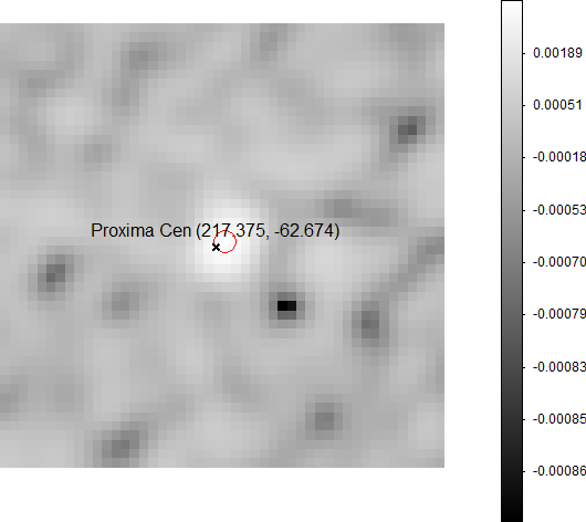
Using NASA Exoplanet Archive data from 29 April 2024 and CASDA catalogue component data from 6 May 2024, we identified 123 likely candidates for exoplanet radio emission. Crossmatching detected two candidate systems: Au Microscopii and Proxima Centauri. Scheduling block ID (SBID) uniquely identifies an ASKAP observation.
| SBID | Separation (arcsec) | Source RA (deg) | Source DEC (deg) | Freq. (MHz) | Peak flux (mJy/beam) | Integrated flux (mJy) | Epoch |
|---|---|---|---|---|---|---|---|
| 50381 | 0.862668 | 217.37493 ± 0.00003 | −62.67425 ± 0.00004 | 887.5 | 9.5 ± 0.2 | 9.7 ± 0.4 | 5 Jun 2023 |
| 52293 | 2.968956 | 217.37388 ± 0.00008 | −62.67401 ± 0.00010 | 887.5 | 4.7 ± 0.2 | 5.0 ± 0.4 | 30 Aug 2023 |
Figure 8. Detections from the Proxima Centauri system.
| SBID | Separation (arcsec) | Source RA (deg) | Source DEC (deg) | Freq. (MHz) | Peak flux (mJy/beam) | Integrated flux (mJy) | Epoch |
|---|---|---|---|---|---|---|---|
| 36300 | 0.630972 | 311.29175 ± 0.00005 | −31.34313 ± 0.00006 | 1655.5 | 2.41 ± 0.16 | 2.7 ± 0.3 | 22 Jan 2022 |
| 21373 | 1.240632 | 311.29149 ± 0.00017 | −31.34318 ± 0.00017 | 1367.5 | 0.96 ± 0.16 | 1.0 ± 0.3 | 16 Jan 2021 |
| 54320 | 2.104740 | 311.29127 ± 0.00013 | −31.34353 ± 0.00012 | 887.5 | 1.56 ± 0.11 | 2.3 ± 0.3 | 28 Oct 2023 |
Figure 9. Detections from the Au Microscopii system.
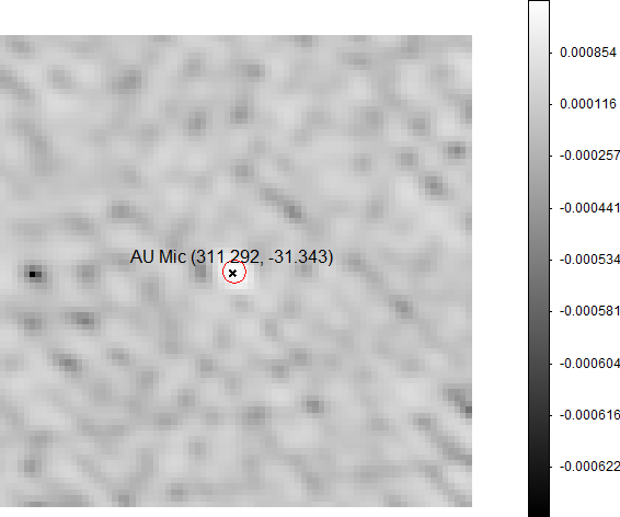
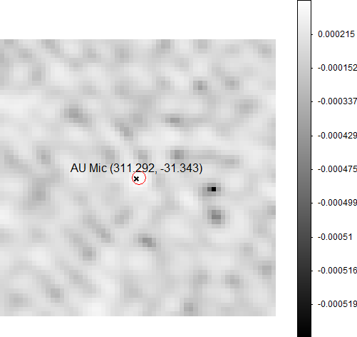
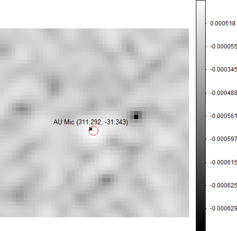
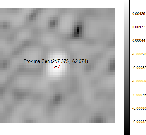
We examined FITS files for the corresponding detections using SAOImageDS9.
4. Discussion
4.1 Proxima Centauri detections
We found two CASDA radio matches for Proxima Centauri b, spaced three months apart and detected at the same frequency, with a large discrepancy between peak and integrated flux values. Proxima Centauri has a mass of , radius of , luminosity of , temperature of , and distance of from Earth [15].
Because Proxima Centauri is a known radio-emitting star, our measurements superimpose the flux of the star and Proxima Centauri b. The inverse-square law means we expect higher readings than for the Au Microscopii system, which is 9.7 pc from Earth.
Proxima Centauri has quiescent emission of approximately 5 mJy near 888 MHz, consistent with both peak and integrated flux measured on 30 August 2023 [19]. Assuming similar quiescent emission for the 5 June 2023 reading, its flux is within one order of magnitude of the theoretical ECMI flux density of approximately 1 mJy for exoplanets orbiting Proxima Centauri [18]. This suggests that exoplanet–star ECMI interaction may cause the elevated flux, though random stellar flux fluctuations from space-weather phenomena cannot be ruled out [19].
4.2 Au Microscopii detections
We found three CASDA radio matches for Au Microscopii b, each about a year apart and detected at different frequencies, with a large discrepancy between peak and integrated flux across observations. Au Microscopii has a mass of , radius of , luminosity of , temperature of , and distance of from Earth [4].
Au Microscopii is a known radio-emitting star with stochastic quiescent emission of approximately 0–4 mJy, consistent with all three detections [2]. The theoretical ECMI flux density for exoplanets orbiting Au Microscopii is approximately – within frequency bounds of approximately –. Although the predictions agree with all three detections, we cannot conclude that the flux is caused by exoplanetary ECMI due to the predictions’ large uncertainties [9].
4.3 Future research
Crossmatching the entire NASA database could identify more candidate systems. Examining circular-polarization data for each matching SBID and comparing it with total intensity would reveal the fractional circular polarization of the radio source. High fractional circular polarization could indicate exoplanet emission and eliminate synchrotron radio sources.
Longer observations of candidates such as Proxima Centauri and Au Microscopii could identify periodicity matching an exoplanet’s orbital period. Together with high fractional circular polarization, this may point to exoplanetary ECMI emission.
5. Conclusion
Exoplanets are of great interest due to their potential habitability, but current detection methods reveal little about it. Radio detection can directly reveal information about planetary magnetic fields and stellar radiative flux, which help determine whether liquid water could exist.
By crossmatching 123 likely radio-emitting exoplanets selected using Hot Jupiter criteria from the NASA Exoplanet Archive with ASKAP survey data, we identified two candidate systems hosting radio-emitting exoplanets. Proxima Centauri and Au Microscopii both exhibit radio flux within predicted ranges for electron-cyclotron maser instability.
Longer observations and measurements in different polarizations are required to determine whether this flux comes from a radio-emitting exoplanet or another phenomenon, and to establish radio emission as a viable method for exoplanet discovery.
6. Contributions
I thank Tara Murphy for the opportunity to conduct this research and for their guidance throughout the project. I also acknowledge my group members: Allison Carr implemented multithreading, processed the data, and wrote the initial crossmatch code; Mary Williams filtered the initial NASA archive and produced the DS9 images. I thank Laura Driessen, Manisha Caleb, and Ashna Gulati from the Sydney Institute for Astronomy Radio Transients group for help with crossmatching, proper-motion correction, and operating DS9. My main contribution was incorporating the astroquery CASDA API to automate proper-motion correction and crossmatching. The project code is available on GitHub.
References
- Akeson, R. L., et al. “The NASA Exoplanet Archive: Data and Tools for Exoplanet Research.” PASP 125.930 (2013), 989–999. doi:10.1086/672273.
- Bloot, S., et al. “Phenomenology and periodicity of radio emission from the stellar system AU Microscopii.” 2023. arXiv:2312.09071.
- Ortiz Ceballos, K. N., et al. “A Volume-Limited Radio Search for Magnetic Activity in 140 Exoplanets with the Very Large Array.” 2024. arXiv:2404.16940.
- Donati, J.-F., et al. “The magnetic field and multiple planets of the young dwarf AU Mic.” MNRAS 525.1 (2023), 455–475. doi:10.1093/mnras/stad1193.
- Driessen, L. N., et al. “Detection of radio emission from stars via proper-motion searches.” PASA 40 (2023), e036. doi:10.1017/pasa.2023.26.
- Fujii, Y., et al. “Radio Emission from Red-Giant Hot Jupiters.” ApJ 820.2 (2016), 122. doi:10.3847/0004-637X/820/2/122.
- Huynh, M., et al. “The CSIRO ASKAP Science Data Archive.” Astronomical Data Analysis Software and Systems XXVII, vol. 522 (2020), 263.
- Wright, J. T., and Gaudi, B. S. “Exoplanet Detection Methods.” 2012. doi:10.48550/arXiv.1210.2471.
- Kavanagh, R. D., et al. “Planet-induced radio emission from the coronae of M dwarfs: the case of Prox Cen and AU Mic.” MNRAS 504.1 (2021), 1511–1518. doi:10.1093/mnras/stab929.
- Ling, J., et al. “Searching for Stellar and Planetary Emission in Large Field-of-view Radio Sky Surveys.” ApJ 926.2 (2022), 228. doi:10.3847/1538-4357/ac4514.
- Lynch, C. R., et al. “The detectability of radio emission from exoplanets.” MNRAS 478.2 (2018), 1763–1775. doi:10.1093/mnras/sty1138.
- McConnell, D., et al. “The Rapid ASKAP Continuum Survey I: Design and first results.” PASA 37 (2020), e048. doi:10.1017/pasa.2020.41.
- Murphy, T., et al. “Limits on low-frequency radio emission from southern exoplanets with the Murchison Widefield Array.” MNRAS 446.3 (2014), 2560–2565. doi:10.1093/mnras/stu2253.
- Naoz, S., et al. “Hot Jupiters from secular planet–planet interactions.” Nature 473.7346 (2011), 187–189. doi:10.1038/nature10076.
- Ribas, I., et al. “The habitability of Proxima Centauri b: I. Irradiation, rotation and volatile inventory from formation to the present.” A&A 596 (2016), A111. doi:10.1051/0004-6361/201629576.
- Rouan, D. “Proper Motion.” Encyclopedia of Astrobiology (2011), 1345–1347. doi:10.1007/978-3-642-11274-4_1283.
- Lazio, T. J. W., et al. “The Radiometric Bode’s Law and Extrasolar Planets.” ApJ 612.1 (2004), 511. doi:10.1086/422449.
- Turnpenney, S., et al. “Exoplanet-induced Radio Emission from M Dwarfs.” ApJ 854.1 (2018), 72. doi:10.3847/1538-4357/aaa59c.
- Zic, A., et al. “A Flare-type IV Burst Event from Proxima Centauri and Implications for Space Weather.” ApJ 905.1 (2020), 23. doi:10.3847/1538-4357/abca90.