Aside: This article was adapted from the results of my undergraduate research. For more background information, see FRB Primer.
Abstract
We compare MeerKAT observations of the repeating fast radio burst FRB121102 from 2019 and 2022. Over this three-year period, the bursts became fainter, their dispersion measure decreased by approximately 10 pc cm−3, and the flux density of the associated persistent radio source also declined. We test whether an expanding supernova remnant could account for the dispersion-measure change, but the model predicts a much shorter timescale than observed. Further monitoring is needed to determine whether the changes originate in the burst source, its local environment, or propagation effects.
1. Introduction
FRB121102 data between 2019–2022 were examined for anomalous readings. This FRB is particularly interesting because it has some unique features. It is a repeating FRB, and the first FRB found to repeat. Since this discovery, it has been monitored by radio telescopes around the world. This heavy monitoring allowed it to be localized very precisely to a dwarf star-forming galaxy. While it does not have a short-timescale period between repeat bursts, it does appear to have a long-term activity period of around 160 days.
Crucially, FRB121102 is also one of only two of the 3,000-odd known FRBs to be co-localised with a persistent radio source (PRS). This associated PRS is central to our research, as we aim to investigate whether the PRS and the FRB are causally connected, and whether this could tell us more about FRB production in general.
2. Methods
2.1 MeerKAT observations
We compared detections of bursts from FRB121102 in 2019 and 2022. The 2022 plots use a darker colour map to emphasize the bursts because they are fainter.
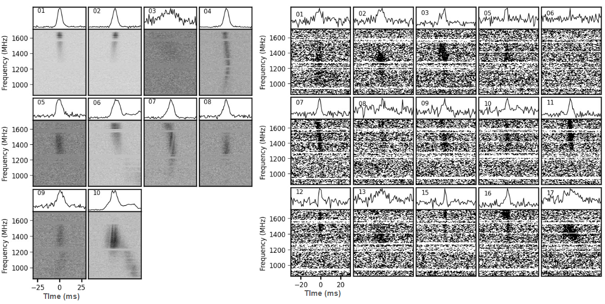
These plots let us visualize the features of each burst and compare the two sets of detections. Their frequency range, 856–1,712 MHz, is the bandwidth of the MeerKAT telescope. In each plot:
- The top section is the signal’s time series: the dedispersed signal averaged over all frequency channels to produce a peak.
- The bottom section is the signal’s waterfall plot after dedispersion.
All detections were made with the MeerKAT telescope in South Africa using the same calibrations and configuration. The only difference between the two sets of measurements was the three-year interval. We analyzed the data using DM_phase and mtcutils, then aggregated the results into these plots.
2.2 Dispersion-measure analysis
We filtered the data for bursts with a signal-to-noise ratio above 10, the historical threshold for treating a signal as believable rather than noise. We then compared the median signal-to-noise-maximizing DM (S/N DM) and structure-maximizing DM (SM DM) from 2019 and 2022.
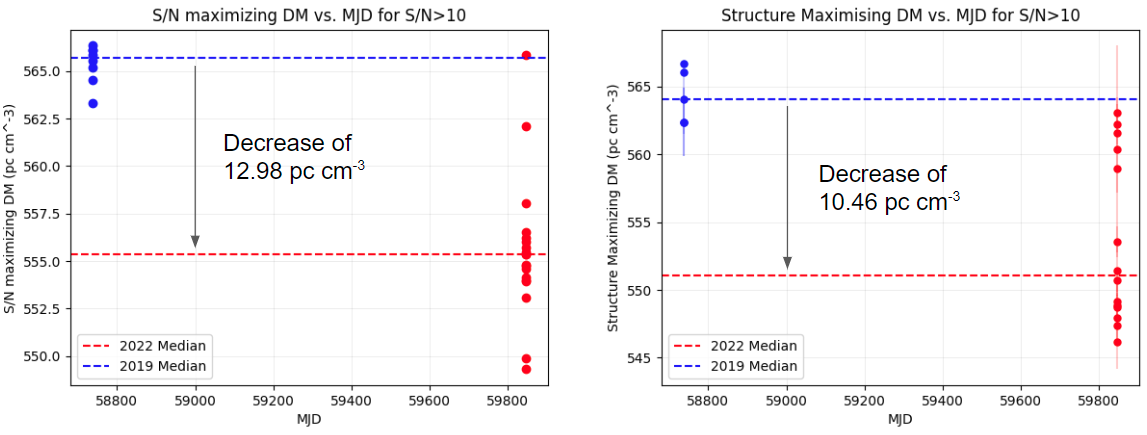
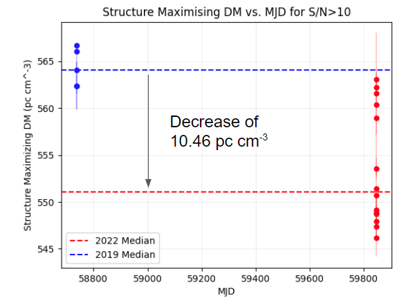
Both measures show a DM decrease of approximately 10 pc cm−3 over three years.
3. Results
The main differences between the 2019 and 2022 MeerKAT detections are summarized below.
| Parameter | 2019 | 2022 | Difference |
|---|---|---|---|
| Median S/N | 85.02 | 14.60 | −70.42 |
| Median S/N DM | 567.62 pc cm−3 | 557.54 pc cm−3 | −10.46 pc cm−3 |
| Median SM DM | 564 ± 3 pc cm−3 | 551 ± 1 pc cm−3 | −13 ± 4 pc cm−3 |
| PRS flux density | 269 µJy | 189 µJy | −80 µJy |
Table 1. Summary of FRB121102 changes from 2019 to 2022.
We focused on time-series data rather than imaging data. The flux-density values for the PRS associated with FRB121102 therefore came from imaging observations taken simultaneously with the 2019 and 2022 MeerKAT time-series data. These values were published in a 2023 paper.
Uncertainties are included for median SM DM, provided by DM_phase, because this measure describes the burst structure of interest. S/N DM uncertainties are not included because they are not relevant to this research; the appendix outlines how they could be calculated.
In summary, we found:
- A decrease in the bursts’ signal-to-noise ratio.
- A decrease of around 10 pc cm−3 in both structure-maximizing and signal-to-noise-maximizing dispersion measures.
- A decrease in the flux density of the PRS associated with the FRB.
The DM decrease was also confirmed by the FAST telescope in China through observations made independently and simultaneously with MeerKAT.
4. Discussion
4.1 Comparison with pulsars
This change in DM had not been observed in another FRB, so we looked to a related class of source—pulsars—for possible explanations. Pulsar DMs are known to vary over time, but surveys over comparable timescales show decreases several orders of magnitude below the change in FRB121102.
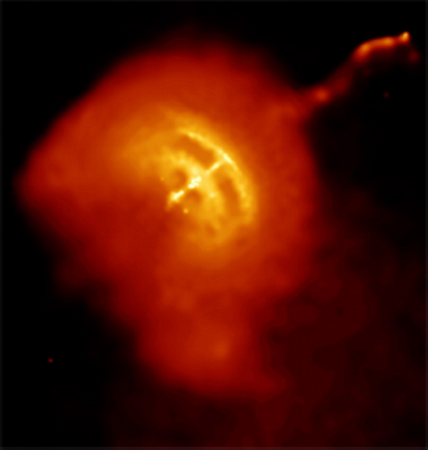
For example, the Vela Pulsar was observed at multiple frequencies for six years and showed a relatively extreme pulsar DM decrease of 0.005 pc cm−3 per year. This is still far below the approximately 10 pc cm−3 decrease observed for FRB121102 over three years.
This suggests that the change likely occurred in the source producing FRB121102 rather than along its line of sight. In particular, a change in the associated PRS could have produced both the DM and flux-density decreases.
4.2 Supernova-remnant model
One possible FRB progenitor model places the PRS inside a supernova remnant (SNR) that expands over time. An SNR is the material left by a star’s explosion at the end of its life, such as the Crab Nebula.
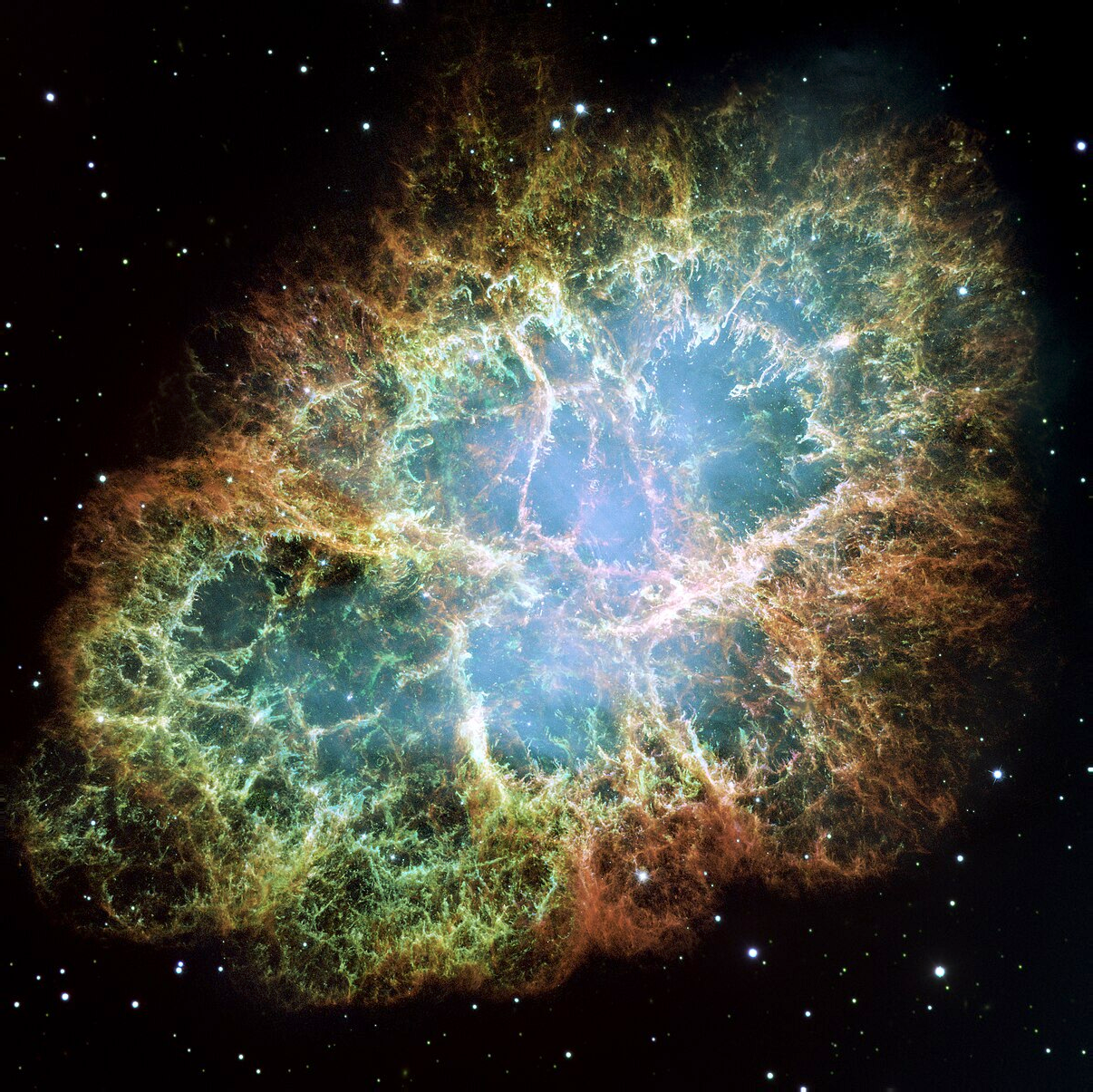
We tested whether an expanding remnant could explain the DM decrease between 2019 and 2022. As the remnant expands, its gas becomes less dense and its associated dispersion measure should decrease. We modeled two scenarios:
- A core-collapse supernova, caused by a massive star at the end of its life.
- A Type Ia supernova, caused when a white dwarf accretes too much mass from an orbiting star.
For each scenario we tested stripped and non-stripped models. The stripped model assumes that most of the source star’s mass has been blown away; the non-stripped model assumes that most of it remains.
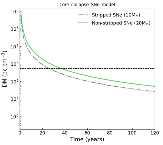
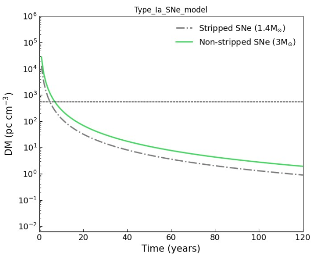
Each graph shows DM as a function of time predicted by the model. We varied the initial masses and ejection speeds of the remnants. The horizontal dashed lines indicate the measured FRB121102 DM values in 2019 and 2022.
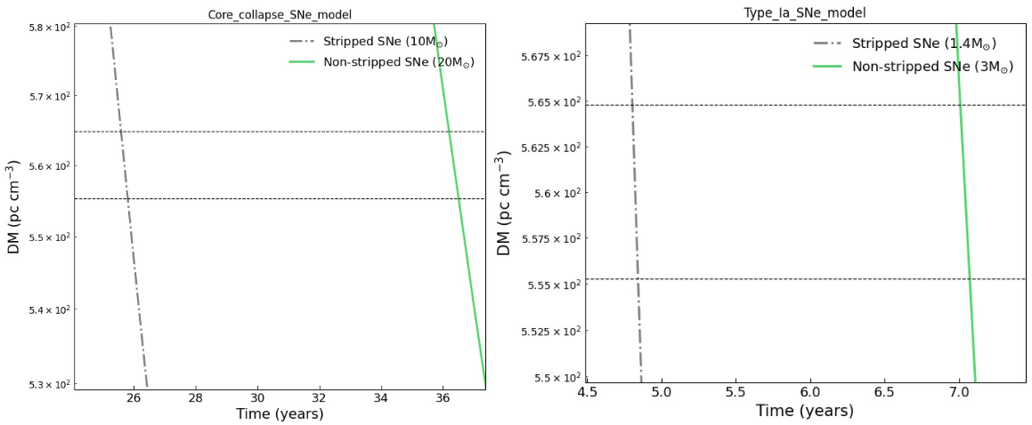
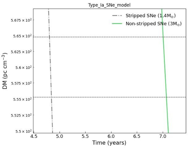
According to the models, the expected time required for the observed 10 pc cm−3 decrease is:
| Model | Core collapse | Type Ia |
|---|---|---|
| Stripped | 0.22 years | 0.034 years |
| Non-stripped | 0.32 years | 0.064 years |
Table 2. Expected duration of the measured DM decrease.
These durations are only a small fraction of the actual three-year observation interval. Although the models offer a mechanism for decreasing DM, their timescales do not match our observations, so the observed change cannot be fully explained by this SNR expansion model.
5. Conclusion
Significant changes were found in the FRB121102 burst detections between 2019 and 2022. In particular, the decrease in DM had not been seen elsewhere in the known FRB population, potentially allowing us to constrain FRB progenitor models in a new way.
The SNR expansion model examined here does not fully explain the observed changes. Future observations are needed to determine whether scintillation caused the PRS flux-density changes or whether they were intrinsic to the source, and whether the activity of the FRB and PRS are correlated. An accepted proposal will observe FRB121102 for 73 hours over a 12-month period with MeerKAT, allowing these changes to be investigated further.
We hope that these observations take us one step further toward answering the questions surrounding the production of FRB121102 and FRBs in general. For now, fast radio bursts remain a fascinating enigma.
Acknowledgements
I would like to thank Dr. Manisha Caleb and the Radio Transients group from the Sydney Institute for Astronomy (SIfA) for their invaluable guidance and support throughout this project. Special thanks go to my colleague Mary Williams for our fruitful collaboration.
This project relied on the DM_phase program, authored by Daniele Michilli, Andrew Seymour, and Ziggy Pleunis, and the mtcutils program by Vincent Morello. I also acknowledge the essential contribution of the MeerKAT radio telescope in South Africa, which provided the raw data used in this study.
Appendix: Signal-to-noise DM uncertainties
In principle, signal-to-noise DM uncertainty can be calculated using the DM curve provided by mtcutils:
- Find the peak S/N value.
- Find where the DM curve intersects a horizontal line at peak S/N minus one.
- Record the DM values at the two intersections.
- Take the difference between those values as the S/N DM uncertainty.
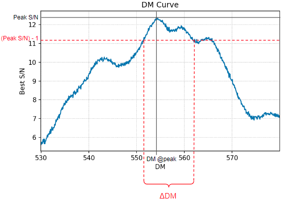
mtcutils, illustrating the signal-to-noise DM uncertainty calculation.